Back to the Basics: Essential Statistics for Data Science

As a computer science student specializing in AI, I believe that having a strong foundation in any subject is key to succeeding in a constantly evolving learning journey. To help myself remember these fundamental concepts and hopefully help some of you as well I’ve put together this recap of basic Statistics for Data Science.

This is also part of my own revision journey, as I revisit the fundamentals and strengthen my understanding of the basics.

1. Understanding Your Data: Types & Structures

Before running any predictive models or writing a single line of Python, you need to understand the shape and type of your data.

In data science, we generally work with Structured Data (tables, rows, columns like a PostgreSQL database) or Unstructured Data (rich media like images or audio that require heavy preprocessing).

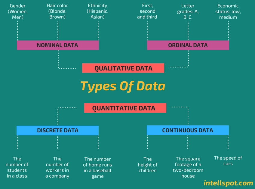
• Qualitative (Categorical) Data:

  • Nominal: Categories with no inherent order or ranking.

    • Example: Audio classification labels (e.g., "Siren", "Speech", "Dog Barking") in an environmental sound alert app.

  • Ordinal: Categories with a meaningful order or ranking.

    • Example: Risk categories in a student dropout prediction model (e.g., "Low Risk", "Medium Risk", "High Risk").

• Quantitative (Numerical) Data:

  • Discrete: Countable numerical values, typically representing whole-number counts.

    • Example: The number of images stored in a local SQLite gallery database.

  • Continuous: Numerical measurements that can take any value within a range, including decimals.

    • Example: Joint coordinates and knee-bend angles calculated using MediaPipe during a squat form analysis.

2. Population vs. Sampling in Machine Learning

In statistics, the population refers to the entire group of data points we want to study. However, processing an entire population is usually computationally expensive and impractical.

Instead, we use a sample a representative subset of the population. In data science, this concept is directly tied to how we split our datasets (like using train_test_split in Scikit-Learn).

Key probability sampling methods include:

• Simple Random Sampling: Every data point has an equal chance of being selected (e.g., randomly shuffling a Pandas DataFrame).

• Stratified Sampling: Dividing the population into subgroups (strata) and randomly sampling from each. Example: Ensuring your training data has an equal proportion of all facial recognition subjects to prevent a biased model.

3. Descriptive Statistics: Measures of Central Tendency

Descriptive statistics organize and summarize the main features of a dataset. The most common way to summarize data is by finding its center.

• Mean: The arithmetic average. It is easily affected by outliers.

  $$\bar{x} = \frac{\sum_{i=1}^{n} x_i}{n}$$

  • Example: The average price of tomatoes over a month in a Kalimati market dataset.

• Median: The exact middle value when data is sorted. It is highly robust to outliers because when data is sorted the outliers lie either on the left most or the right most side.

• Mode: The most frequent value, typically used for categorical data.

4. Measures of Dispersion: Understanding the Spread

Two datasets can have the exact same mean but look completely different. Dispersion tells us how spread out our data points are from the center.

• Range: The difference between the maximum and minimum values.

• Percentile: Divides the data into 100 equal parts. For example, the 25th percentile means that 25% of the data lies below that specific value. (Note: The 50th percentile is exactly the same as the median).

• Quartiles: Divides the data into four equal parts.

  

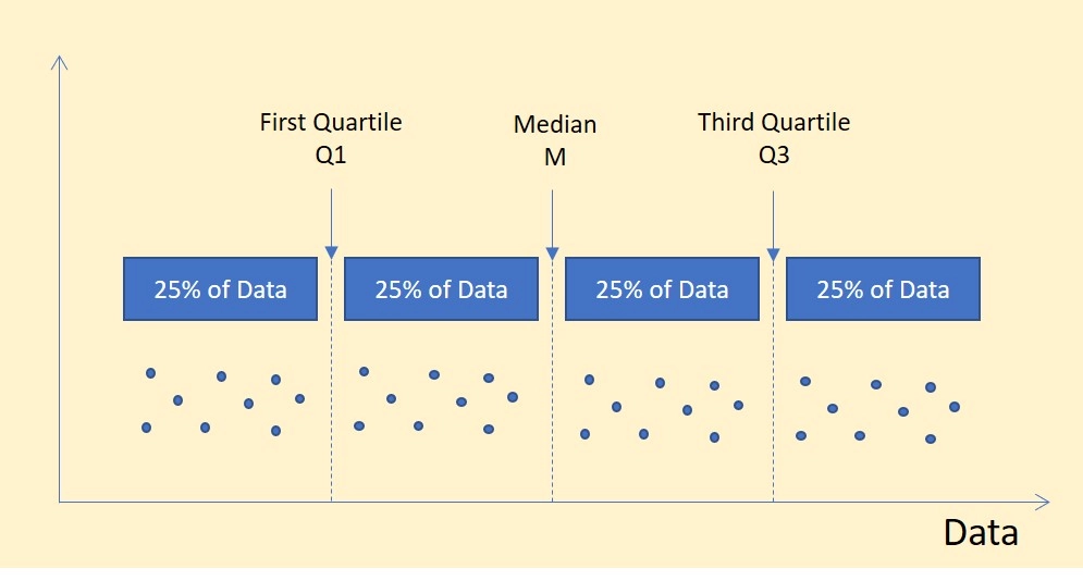
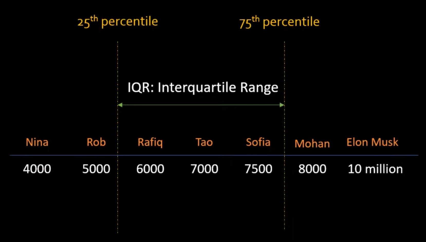
• Interquartile Range (IQR): Measures the spread of the middle 50% of your data, ignoring extremes.

$$IQR = Q3 - Q1$$

(where Q3 is the 75th percentile and Q1 is the 25th percentile).

• Variance: The average of the squared differences from the mean. We square the values so positive and negative deviations don't cancel each other out to zero, and to give more weight to extreme values.

  $$\sigma^2 = \frac{1}{n}\sum_{i=1}^{n}(x_i-\mu)^2 \qquad\text{(Variance)}$$

• Standard Deviation: The square root of the variance. This converts the measurement back to the original units of the data.

  $$\sigma = \sqrt{\frac{1}{n}\sum_{i=1}^{n}(x_i-\mu)^2} \qquad\text{(Standard Deviation)}$$

• Both Variance and Standard Deviation measures spread but Variance is harder to interpret as it is squared. We square the differences in Variance to avoid negative value and emphasize larger deviations. Standard deviation on the other hand is easier to interpret because it's in the original units of the data.

5. Identifying Outliers

Outliers are data points that deviate significantly from the rest of the dataset. In machine learning, outliers can completely ruin a regression model if not handled properly.

There are two primary mathematical ways to detect them:

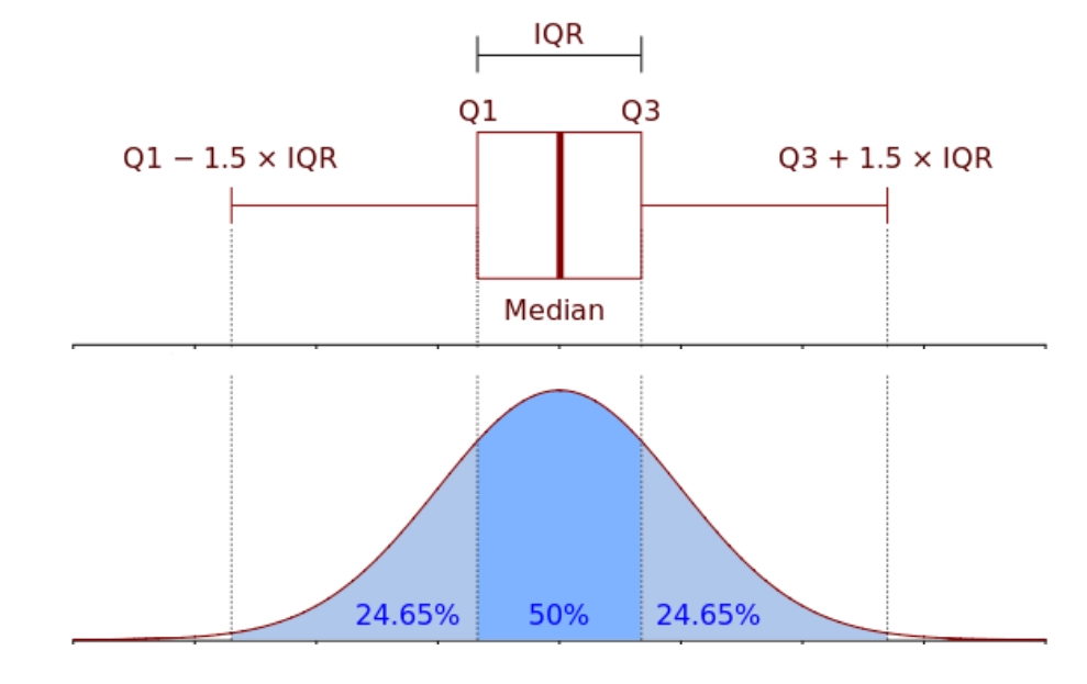
1. The IQR Method (Used in Box Plots): A data point is an outlier if it falls outside these boundaries:

   $$\text{Lower Limit} = Q_1 - 1.5(IQR)$$

$$\text{Upper Limit} = Q_3 + 1.5(IQR)$$

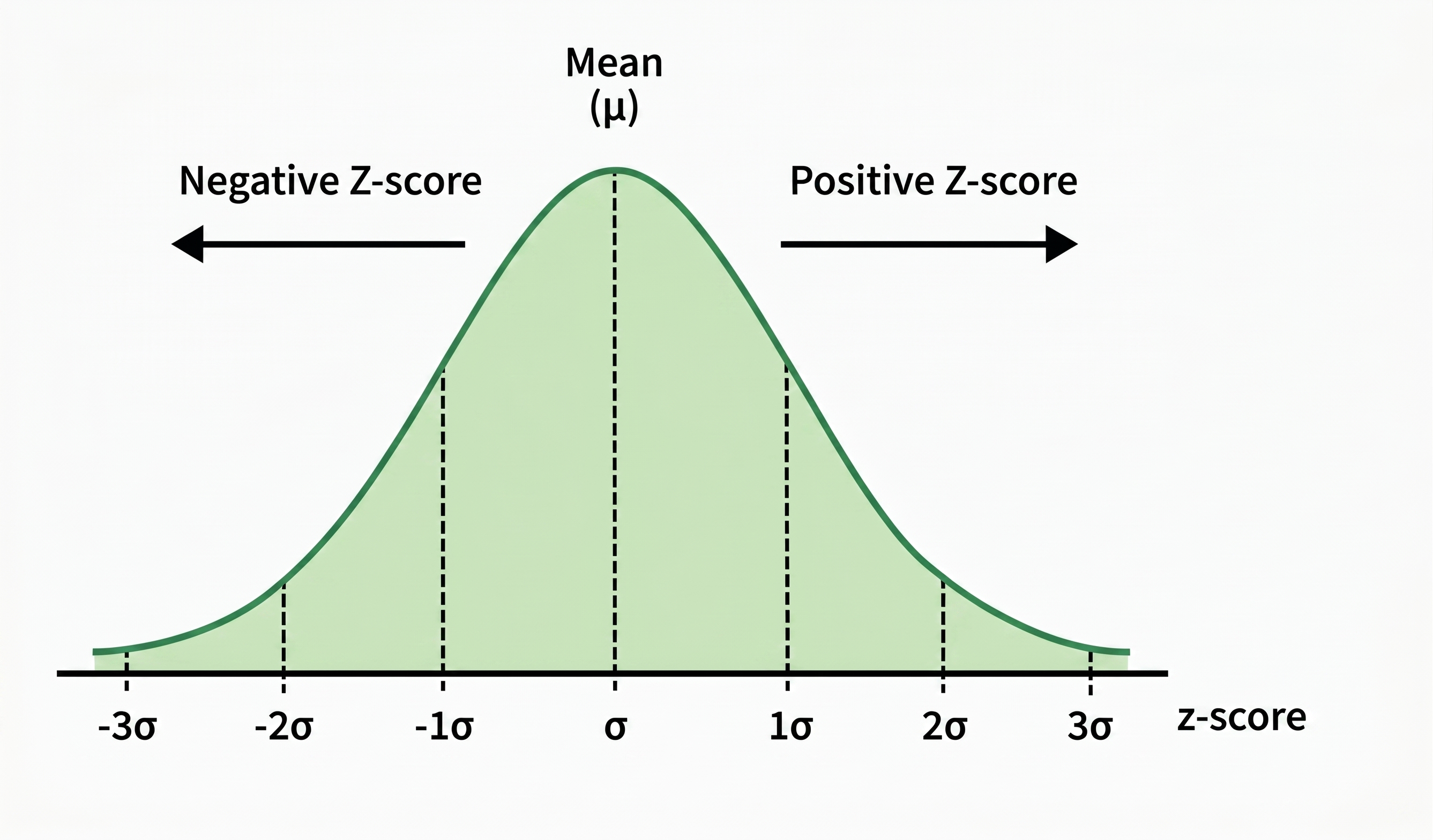
1. The Z-Score Method: This measures exactly how many standard deviations a data point is away from the mean. A Z-score beyond +3 or -3 is generally considered an outlier.

$$Z = \frac{x - \mu}{\sigma}$$

6. Relationships: Covariance & Correlation

When dealing with multivariate data, we need to know how features interact with each other.

• Covariance: Describes the direction of the relationship between two variables (e.g., if feature A increases, does feature B increase?).

$$\operatorname{Cov}(X,Y) = \frac{1}{n}\sum_{i=1}^{n}(x_i-\bar{x})(y_i-\bar{y}) \qquad\text{(Covariance)}$$

• Correlation: Measures both the direction and the strength of a linear relationship on a scale from -1 to 1.

  $$r = \frac{\operatorname{Cov}(X,Y)}{\sigma_X\sigma_Y} \qquad\text{(Correlation)}$$

  • r = 1: Perfect positive correlation.

  • r = -1: Perfect negative correlation.

• r = 0: No linear correlation.

• Causation: Just because two variables correlate does not mean one causes the other. Causation explicitly means a change in one variable is directly responsible for a change in another.

---

Wrapping Up

Having a firm grasp of these mathematical foundations is critical for further learning. The concepts and formulas above are compiled from my personal notes, various blogs, YouTube videos, and college lectures.

I hope this serves as a reminder to me and others that going back to the basics is never something to hesitate about. A strong understanding of the fundamentals makes it much easier to build and understand more advanced concepts.